library(readr)
library(dplyr)
library(ggplot2)
cases <- read_csv("datasets/COVID19_countries_data.csv")
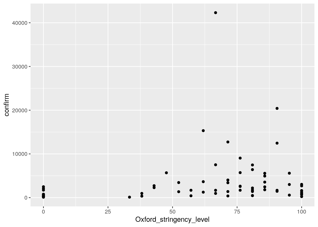
ggplot(cases, aes(Oxford_stringency_level, confirm))+
geom_point()
#ggsave("wrap_up_stats/cases_vs_oxford_scatter.png")
model <- lm(confirm ~ Oxford_stringency_level, cases)
#summary view
summary(model)
##
## Call:
## lm(formula = confirm ~ Oxford_stringency_level, data = cases)
##
## Residuals:
##    Min     1Q Median     3Q    Max
##  -4554  -2532  -1452    168  38591
##
## Coefficients:
##                         Estimate Std. Error t value Pr(>|t|)
## (Intercept)              1571.03    1503.74   1.045    0.300
## Oxford_stringency_level    32.16      21.32   1.509    0.136
##
## Residual standard error: 6012 on 66 degrees of freedom
## Multiple R-squared:  0.03334,    Adjusted R-squared:  0.01869
## F-statistic: 2.276 on 1 and 66 DF,  p-value: 0.1362
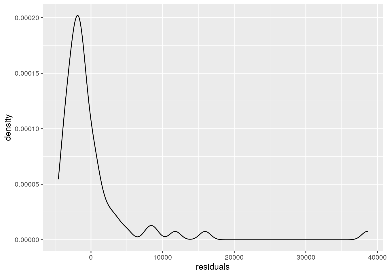
#inspecting whether the residuals are normal distributed
#density distributions of the residuals
cases <- cases %>%
  mutate(residuals = resid(model))
cases %>%
  ggplot(aes(residuals)) +
  geom_density()
#ggsave("wrap_up_stats/residual_density.png")
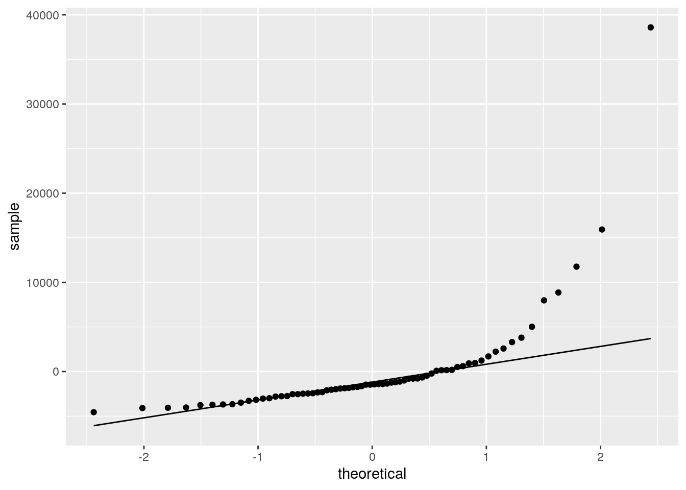
#qq plot of the residuals
ggplot(cases, aes(sample = residuals)) +
  geom_qq() +
  geom_qq_line(distribution = qnorm)
ggsave("wrap_up_stats/qqplot_residuals.png")
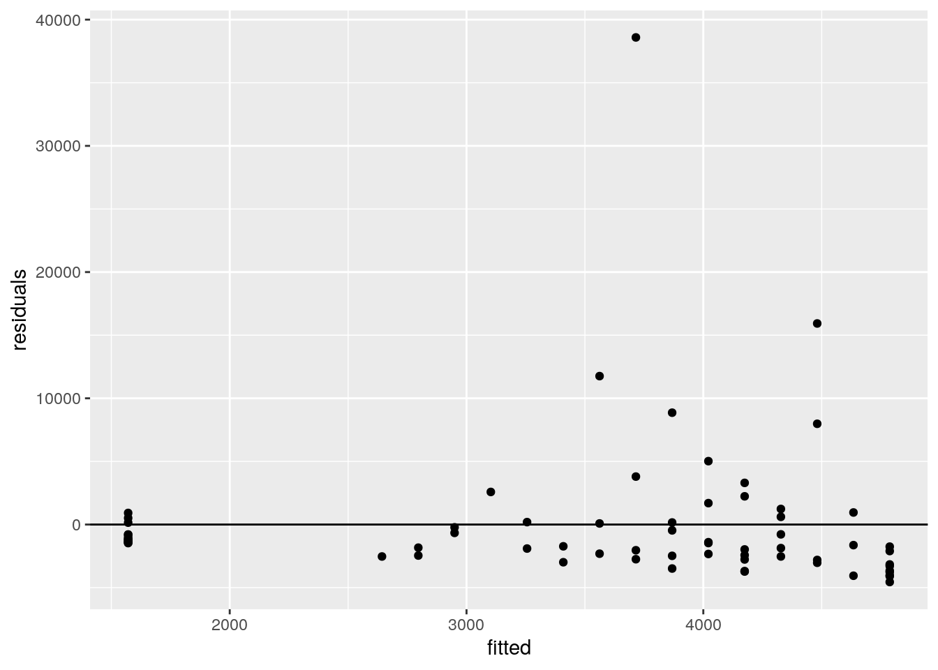
#looking at the residuals vs. the fitted values
cases <- cases %>%
  mutate(fitted = fitted(model))
ggplot(cases, aes(fitted, residuals)) +
  geom_point() +
  geom_hline(yintercept = 0)
ggsave("wrap_up_stats/residual_vs_fitted.png")
#Data points with fitted regression line
ggplot(cases, aes(Oxford_stringency_level, confirm))+
  geom_point()+
  geom_abline(intercept = 1571, slope = 32.2)
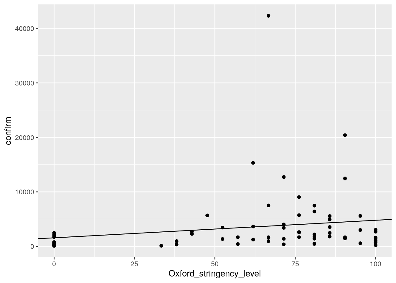
ggsave("wrap_up_stats/cases_oxford_stringency_scatter_w_regression.png")

#direct geom_smooth way
ggplot(cases, aes(Oxford_stringency_level, confirm))+
  geom_point() +
  geom_smooth(method = "lm")
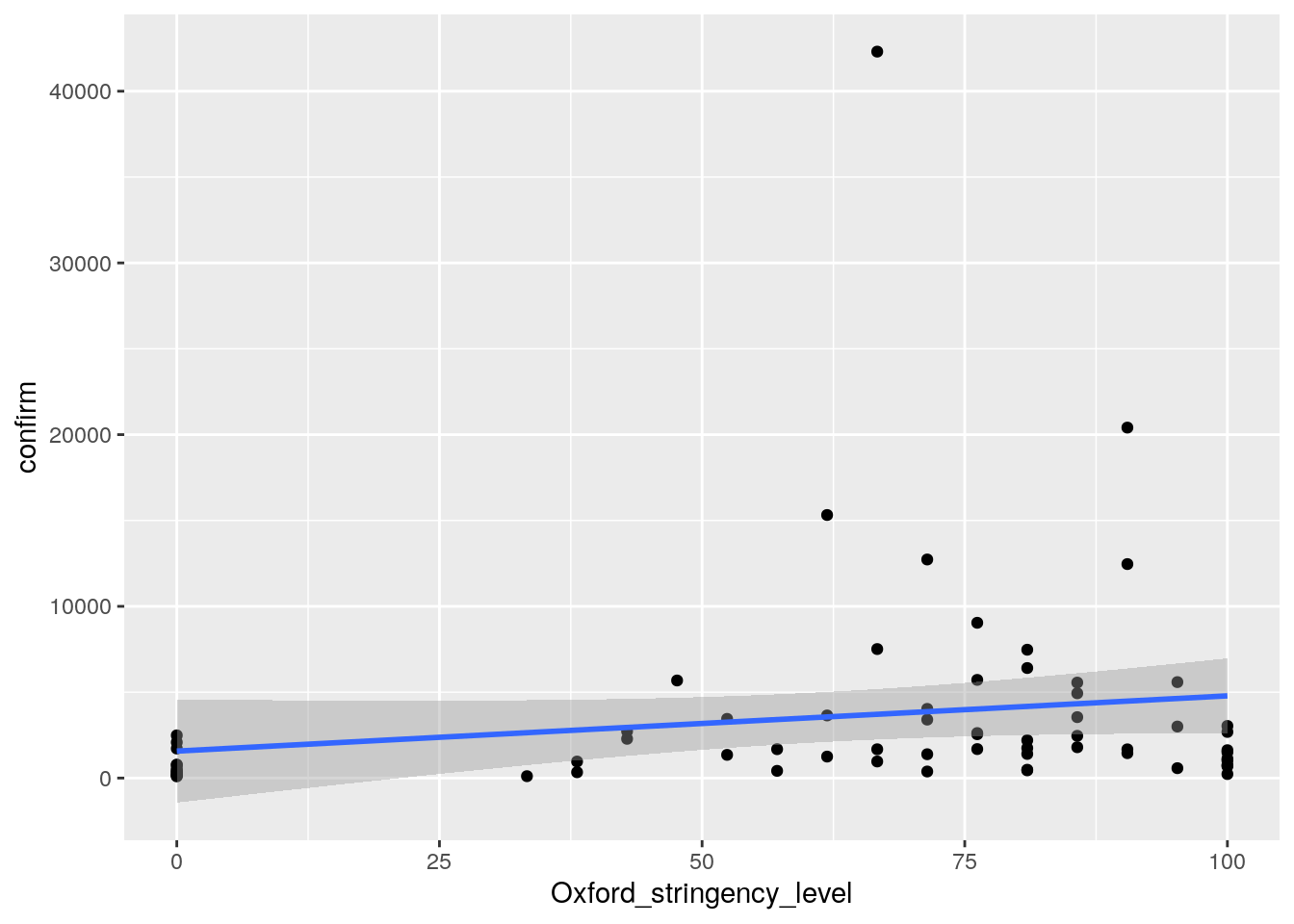
ggsave("wrap_up_stats/cases_oxford_stringency_scatter_w_regression_v2.png")
model2 <- lm(confirm ~ Oxford_stringency_level +  tourist_departure_2018, cases)
summary(model2)
##
## Call:
## lm(formula = confirm ~ Oxford_stringency_level + tourist_departure_2018,
##     data = cases)
##
## Residuals:
##     Min      1Q  Median      3Q     Max
## -9138.6 -1624.8  -556.4  1617.7 14881.7
##
## Coefficients:
##                           Estimate Std. Error t value Pr(>|t|)
## (Intercept)             -1.410e+03  1.384e+03  -1.019   0.3139
## Oxford_stringency_level  3.263e+01  1.910e+01   1.708   0.0948 .
## tourist_departure_2018   2.085e-04  2.190e-05   9.521 3.74e-12 ***
## ---
## Signif. codes:  0 '***' 0.001 '**' 0.01 '*' 0.05 '.' 0.1 ' ' 1
##
## Residual standard error: 3999 on 43 degrees of freedom
##   (22 observations deleted due to missingness)
## Multiple R-squared:  0.6893, Adjusted R-squared:  0.6749
## F-statistic: 47.71 on 2 and 43 DF,  p-value: 1.214e-11
library(broom)
tidy(model)
## # A tibble: 2 x 5
##   term                    estimate std.error statistic p.value
##   <chr>                      <dbl>     <dbl>     <dbl>   <dbl>
## 1 (Intercept)               1571.     1504.       1.04   0.300
## 2 Oxford_stringency_level     32.2      21.3      1.51   0.136
tidy(model2)
## # A tibble: 3 x 5
##   term                        estimate    std.error statistic  p.value
##   <chr>                          <dbl>        <dbl>     <dbl>    <dbl>
## 1 (Intercept)             -1410.       1384.            -1.02 3.14e- 1
## 2 Oxford_stringency_level    32.6        19.1            1.71 9.48e- 2
## 3 tourist_departure_2018      0.000209    0.0000219      9.52 3.74e-12
#direct geom_smooth way
ggplot(cases, aes(tourist_departure_2018, confirm))+
  geom_point() +
  geom_smooth(method = "lm")
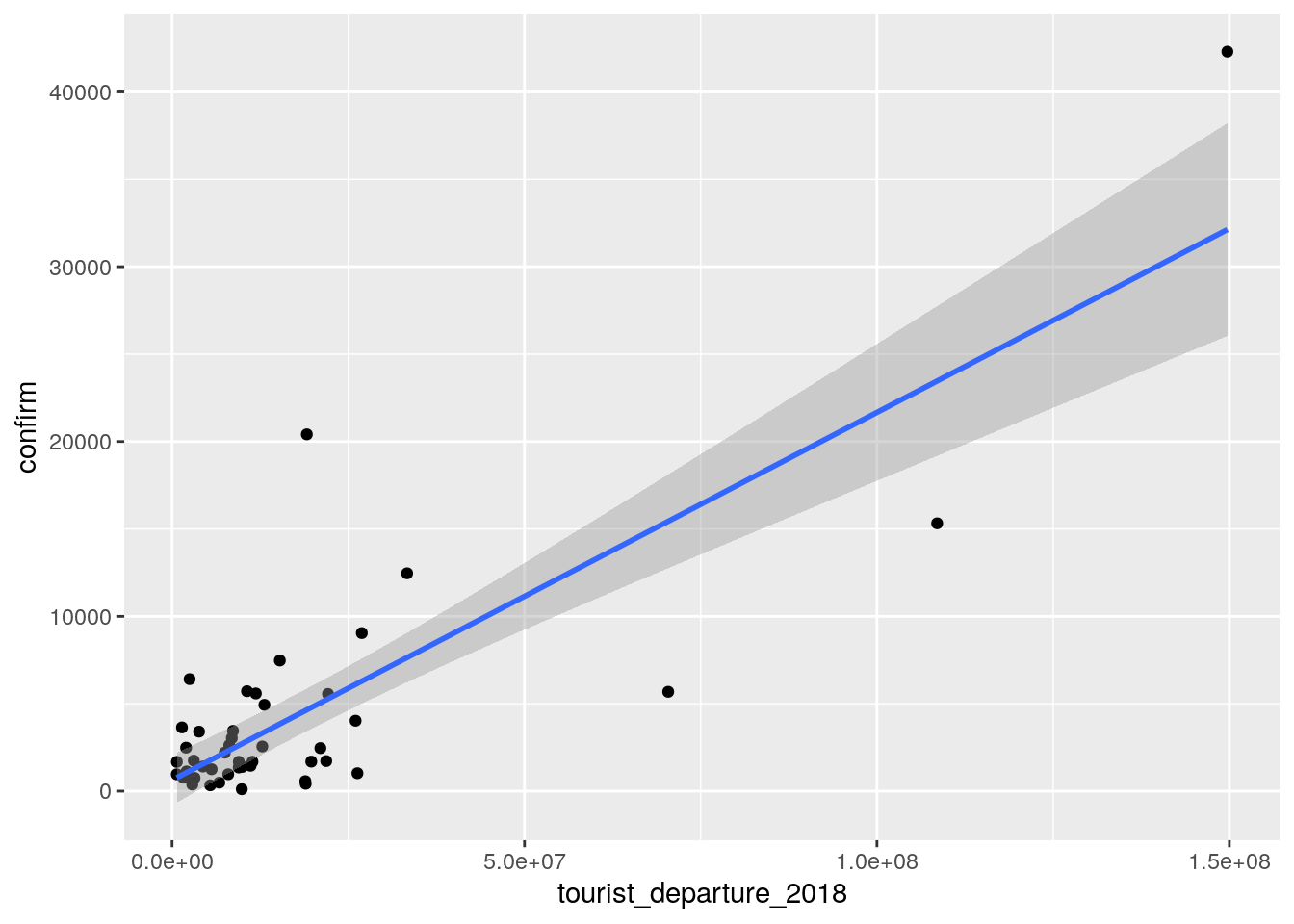
ggsave("wrap_up_stats/cases_vs_tourist_departure.png")